趁五一假期,再写一篇用Tensorflow实现交通标志识别。
今天的任务是通过Tensorflow搭建一个机器学习模型,通过训练来实现识别交通标志。
Python版本:3.5.3
Tensorflow版本:1.0.1
其中还用到了一些其他的库
1 2 3 4 5 6 7 8
| import os import random import skimage.data import skimage.transform import matplotlib import matplotlib.pyplot as plt import numpy as np import tensorflow as tf
|
模型训练和测试用到的数据集来自比利时的交通标志数据集,下载BelgiumTS for Classification (cropped images)中的BelgiumTSC_Training (171.3MBytes) 和 BelgiumTSC_Testing(76.5MBytes),training的数据集用来训练模型,Testing的数据集用来测试模型。
训练集和测试集各包含62个子目录,目录名字是从00000到00061,这些目录代表的是相应交通标志的标签,而每个目录下的图片就是该标签的样本。
首先我们要加载训练数据
数据集中的图片数据是用.ppm格式存储的,可以通过Scikit Image库来读取图片数据
1 2 3 4 5 6 7 8 9 10 11 12 13 14 15 16 17 18 19 20 21 22 23 24
| def load_data(data_dir): """Loads a data set and returns two lists: images: a list of Numpy arrays, each representing an image. labels: a list of numbers that represent the images labels. """ directories = [d for d in os.listdir(data_dir) if os.path.isdir(os.path.join(data_dir, d))] labels = [] images = [] for d in directories: label_dir = os.path.join(data_dir, d) file_names = [os.path.join(label_dir, f) for f in os.listdir(label_dir) if f.endswith(".ppm")] for f in file_names: images.append(skimage.data.imread(f)) labels.append(int(d)) return images, labels
|
加载数据之后返回两个列表,images列表包含图像信息,每个图像信息为numpy数字;labels列表包含列表信息,数值为0到61的整数
然后我们可以看一下一共有多少图像和标签
1 2
| images, labels = load_data(train_data_dir) print("Unique Labels: {0}\n Total Images: {1}".format(len(set(labels)), len(images)))
|
从打印出的结果可以看到,一共有62个标签,4575个训练数据
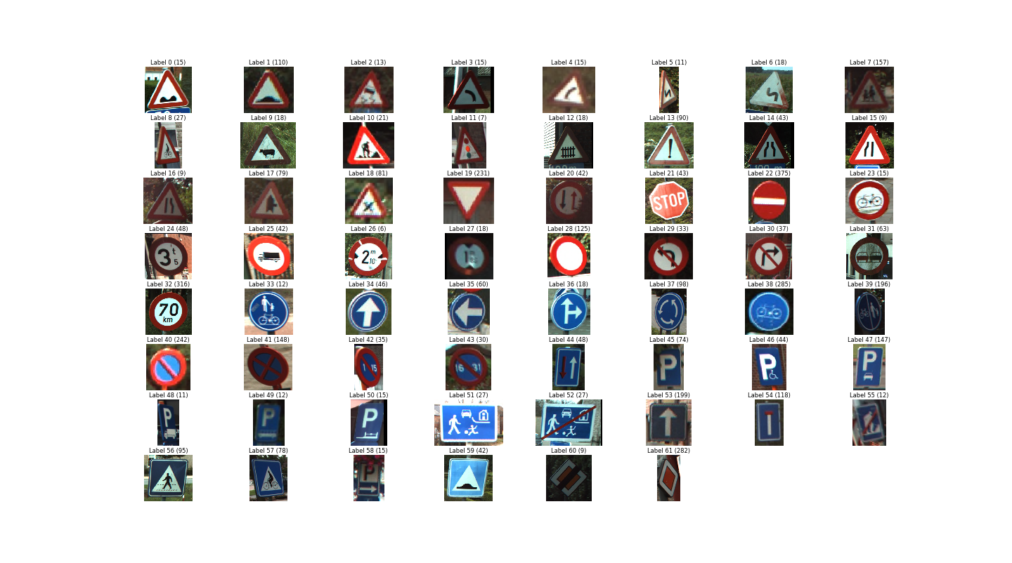
我们可以显示一下每一组标签的第一幅图像
1 2 3 4 5 6 7 8 9 10 11 12 13 14 15 16
| def display_images_and_labels(images, labels): """Display the first image of each label.""" unique_labels = set(labels) plt.figure(figsize=(10, 10),dpi=50) i = 1 for label in unique_labels: image = images[labels.index(label)] plt.subplot(8, 8, i) plt.axis('off') plt.title("Label {0} ({1})".format(label, labels.count(label))) i += 1 _ = plt.imshow(image) plt.show() display_images_and_labels(images, labels)
|
标签和图像信息
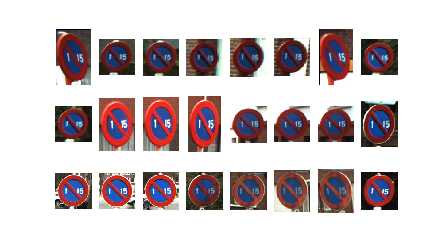
同样,我们也可以显示每一个标签中的图片数据,来看一下第42号标签的数据
1 2 3 4 5 6 7 8 9 10 11 12 13 14 15 16 17
| def display_label_images(images, label): """Display images of a specific label.""" limit = 24 plt.figure(figsize=(15, 5)) i = 1 start = labels.index(label) end = start + labels.count(label) for image in images[start:end][:limit]: plt.subplot(3, 8, i) plt.axis('off') i += 1 plt.imshow(image) plt.show() display_label_images(images, 42)
|
42号标签的图像数据
通过上面的图像显示,我们会发现,这些图片的大小是不一样的。但是大多数的机器学习模型需要输入数据的维数是固定的,因此需要对图像数据进行处理,保证相同的输入数据格式。
1
| images32 = [skimage.transform.resize(image, (32, 32)) for image in images]
|
这样就可以将图片数据转换成32*32*3的图片。
接下来的工作就是搭建神经网络模型
1 2 3 4 5 6 7 8 9 10 11 12 13 14 15 16 17 18 19 20 21 22 23 24 25 26 27 28
| images_ph = tf.placeholder(tf.float32, [None, 32, 32, 3]) labels_ph = tf.placeholder(tf.int32, [None]) images_flat = tf.contrib.layers.flatten(images_ph) logits = tf.contrib.layers.fully_connected(images_flat, 62, tf.nn.relu) predicted_labels = tf.argmax(logits, 1) loss = tf.reduce_mean(tf.nn.sparse_softmax_cross_entropy_with_logits(logits=logits, labels=labels_ph)) train = tf.train.AdamOptimizer(learning_rate=0.001).minimize(loss) init = tf.global_variables_initializer()
|
在模型当中,首先改变一下输入数据的维数,将32*32*3的数据展开成一维的数据(1*3072),然后建立一个3072-62的全连接网络,使用ReLU作为激活函数。用交叉熵作为损失函数,使用ADAM优化器来优化参数,最后初始化模型。
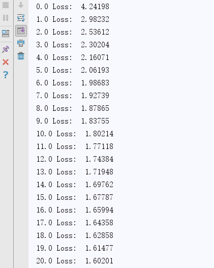
模型搭建好之后,就可以通过训练数据来对模型进行训练,设置训练次数为201次,每训练数次输出一下损失函数的的值
1 2 3 4 5 6 7 8 9 10
| session = tf.Session() _ = session.run([init]) for i in range(201): _, loss_value = session.run([train, loss], feed_dict={images_ph: images_a, labels_ph: labels_a}) if i % 10 == 0: print(i/10,"Loss: ", loss_value)
|
损失函数值
模型训练好之后,既可以用测试数据来见一下模型的性能。
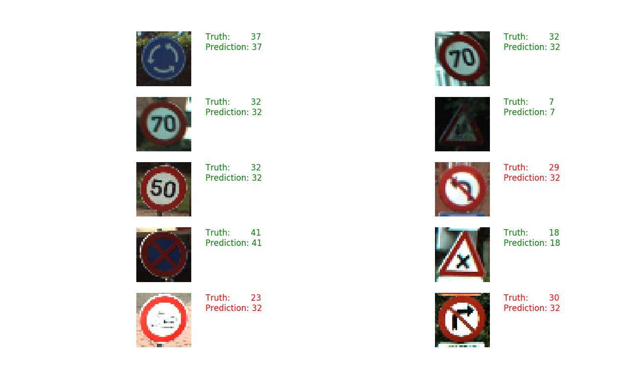
随机抽取测试数据中的10张图片,然后打印出对应的实际标签和识别标签。
1 2 3 4 5 6 7 8 9 10 11 12 13 14 15 16 17 18 19 20 21 22 23 24
| sample_indexes = random.sample(range(len(images32)), 10) sample_images = [images32[i] for i in sample_indexes] sample_labels = [labels[i] for i in sample_indexes] predicted = session.run([predicted_labels], feed_dict={images_ph: sample_images})[0] print(sample_labels) print(predicted) fig = plt.figure(figsize=(10, 10)) for i in range(len(sample_images)): truth = sample_labels[i] prediction = predicted[i] plt.subplot(5, 2,1+i) plt.axis('off') color='green' if truth == prediction else 'red' plt.text(40, 10, "Truth: {0}\nPrediction: {1}".format(truth, prediction), fontsize=12, color=color) plt.imshow(sample_images[i]) plt.show()
|
测试样本
从中可以看到,在10个测试数据中,有7个可以正确识别。
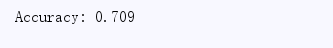
最后,加载所有的测试数据,计算并打印模型的识别正确率。
1 2 3 4 5 6 7 8 9 10 11 12 13 14 15
| test_images, test_labels = load_data(test_data_dir) test_images32 = [skimage.transform.resize(image, (32, 32)) for image in test_images] predicted = session.run([predicted_labels], feed_dict={images_ph: test_images32})[0] match_count = sum([int(y == y_) for y, y_ in zip(test_labels, predicted)]) accuracy = match_count / len(test_labels) print("Accuracy: {:.3f}".format(accuracy))
|
模型识别正确率
可以看出,模型的正确率在70%左右。
参考资料: