之前写了关于DQN(Deep Q Network)的算法分析,今天用Python以及相关的库来设计并实现一个DQN。
本文主要基于OpenAI的开源库gym中的环境再结合TensorFlow来设计与实现DQN。用到了gym中CartPole-v0的立杆子的环境。将每一步得到的状态和奖励值传递给TensorFlow中建立好的QDN网络,并对收集到的状态奖励值进行训练。算法的具体流程参考之前介绍DQN的那篇文章。今天主要介绍代码的实现。
代码主要分为两个部分,首先是建立DQN网络模型,然后导入CartPole-v0环境通过其中返回的状态值和奖励值训练DQN网络。最终实现杆子尽可能长时间地保持不倒。
涉及的主要模块版本号:
Python:3.5.3
TensorFlow:1.0.1
gym:0.8.1
新建DQN.py来建立网络模型以及相关的操作。
首先导入模块以及一些初始设置:
1 2 3 4 5 6
| import numpy as np import pandas as pd import tensorflow as tf np.random.seed(1) tf.set_random_seed(1)
|
然后建立建立DQN模型的类以及一些全局变量:
1 2 3 4 5 6 7 8 9 10 11 12 13 14 15 16 17 18 19 20 21 22 23 24 25 26 27 28 29 30 31 32 33 34 35 36 37 38 39 40 41 42 43 44 45
| class DeepQNetwork: def __init__( self, n_actions, n_features, learning_rate=0.01, reward_decay=0.9, e_greedy=0.9, replace_target_iter=300, memory_size=500, batch_size=32, e_greedy_increment=None, output_graph=False, ): self.n_actions = n_actions self.n_features = n_features self.lr = learning_rate self.gamma = reward_decay self.epsilon_max = e_greedy self.replace_target_iter = replace_target_iter self.memory_size = memory_size self.batch_size = batch_size self.epsilon_increment = e_greedy_increment self.epsilon = 0 if e_greedy_increment is not None else self.epsilon_max self.learn_step_counter = 0 self.cost = 0 self.memory = np.zeros((self.memory_size, n_features * 2 + 2)) self._build_net() self.sess = tf.Session() if output_graph: tf.summary.FileWriter("logs/", self.sess.graph) self.sess.run(tf.global_variables_initializer()) self.cost_his = []
|
self.memory建立一个全0的矩阵用来存储状态和奖励值。大小为500x10(self.memory = 500 ; n_feature*2+2 = 10)。每一行保存当前状态,奖励值,动作,和采取动作之后的下一个状态。self.epsilon表示动作选择时的贪婪值。
然后建立DQN网络,一共需要建立两个网络,一个是目标网络,一个是估计网络,网络的输入为模型中的状态值,输出为动作值,其中包含一个隐藏节点为10的隐藏层。
1 2 3 4 5 6 7 8 9 10 11 12 13 14 15 16 17 18 19 20 21 22 23 24 25 26 27 28 29 30 31 32 33 34 35 36 37 38 39 40 41 42 43 44
| def _build_net(self): self.s = tf.placeholder(tf.float32, [None, self.n_features], name='s') self.q_target = tf.placeholder(tf.float32, [None, self.n_actions], name='Q_target') with tf.variable_scope('eval_net'): c_names, n_l1, w_initializer, b_initializer = \ ['eval_net_params', tf.GraphKeys.GLOBAL_VARIABLES], 10, \ tf.random_normal_initializer(0., 0.3), tf.constant_initializer(0.1) with tf.variable_scope('l1'): w1 = tf.get_variable('w1', [self.n_features, n_l1], initializer=w_initializer, collections=c_names) b1 = tf.get_variable('b1', [1, n_l1], initializer=b_initializer, collections=c_names) l1 = tf.nn.relu(tf.matmul(self.s, w1) + b1) with tf.variable_scope('l2'): w2 = tf.get_variable('w2', [n_l1, self.n_actions], initializer=w_initializer, collections=c_names) b2 = tf.get_variable('b2', [1, self.n_actions], initializer=b_initializer, collections=c_names) self.q_eval = tf.matmul(l1, w2) + b2 with tf.variable_scope('loss'): self.loss = tf.reduce_mean(tf.squared_difference(self.q_target, self.q_eval)) with tf.variable_scope('train'): self._train_op = tf.train.RMSPropOptimizer(self.lr).minimize(self.loss) self.s_ = tf.placeholder(tf.float32, [None, self.n_features], name='s_') with tf.variable_scope('target_net'): c_names = ['target_net_params', tf.GraphKeys.GLOBAL_VARIABLES] with tf.variable_scope('l1'): w1 = tf.get_variable('w1', [self.n_features, n_l1], initializer=w_initializer, collections=c_names) b1 = tf.get_variable('b1', [1, n_l1], initializer=b_initializer, collections=c_names) l1 = tf.nn.relu(tf.matmul(self.s_, w1) + b1) with tf.variable_scope('l2'): w2 = tf.get_variable('w2', [n_l1, self.n_actions], initializer=w_initializer, collections=c_names) b2 = tf.get_variable('b2', [1, self.n_actions], initializer=b_initializer, collections=c_names) self.q_next = tf.matmul(l1, w2) + b2
|
然后创建函数用来保存转移信息(当前状态,动作,奖励,下一个状态):
1 2 3 4 5 6 7 8 9 10
| def store_transition(self, s, a, r, s_): if not hasattr(self, 'memory_counter'): self.memory_counter = 0 transition = np.hstack((s, [a, r], s_)) index = self.memory_counter % self.memory_size self.memory[index, :] = transition self.memory_counter += 1
|
下面建立状态选择函数,函数需要传入当前的状态值用来作为网络的输入,并调用评估网络得到对应的动作:
1 2 3 4 5 6 7 8 9 10 11
| def choose_action(self, observation): observation = observation[np.newaxis, :] if np.random.uniform() < self.epsilon: actions_value = self.sess.run(self.q_eval, feed_dict={self.s: observation}) action = np.argmax(actions_value) else: action = np.random.randint(0, self.n_actions) return action
|
DQN的动作选择采用贪婪策略,$\epsilon$的概率选择动作值函数的最大值,$1-\epsilon$的概率随机选择动作值,这样可以使模型对未知的状态进行探索。
然后建立网络替换函数,当达到一定步数的时候(replace_target_iter =300)需要将估计网络的参数赋给目标网络:
1 2 3 4
| def _replace_target_params(self): t_params = tf.get_collection('target_net_params') e_params = tf.get_collection('eval_net_params') self.sess.run([tf.assign(t, e) for t, e in zip(t_params, e_params)])
|
然后建立学习函数,用来对模型参数进行学习:
1 2 3 4 5 6 7 8 9 10 11 12 13 14 15 16 17 18 19 20 21 22 23 24 25 26 27 28 29 30 31 32 33 34 35 36 37 38
| def learn(self): if self.learn_step_counter % self.replace_target_iter == 0: self._replace_target_params() if self.memory_counter > self.memory_size: sample_index = np.random.choice(self.memory_size, size=self.batch_size) else: sample_index = np.random.choice(self.memory_counter, size=self.batch_size) batch_memory = self.memory[sample_index, :] q_next, q_eval = self.sess.run( [self.q_next, self.q_eval], feed_dict={ self.s_: batch_memory[:, -self.n_features:], self.s: batch_memory[:, :self.n_features], }) q_target = q_eval.copy() batch_index = np.arange(self.batch_size, dtype=np.int32) eval_act_index = batch_memory[:, self.n_features].astype(int) reward = batch_memory[:, self.n_features + 1] q_target[batch_index, eval_act_index] = reward + self.gamma * np.max(q_next, axis=1) _, self.cost = self.sess.run([self._train_op, self.loss], feed_dict={self.s: batch_memory[:, :self.n_features], self.q_target: q_target}) self.cost_his.append(self.cost) self.epsilon = self.epsilon + self.epsilon_increment if self.epsilon < self.epsilon_max else self.epsilon_max self.learn_step_counter += 1
|
代码中,当达到参数替换的迭代数之后(replace_target_iter)需要替换目标网络的参数。然后在状态的存储空间中随机选择训练数据(self.batch_size = 32)。然后调用目标网络和估计网络分别计算当前状态的Q值和下一状态的Q值。在下一状态的Q值中选择最大值并乘以衰减系数$\gamma$加上奖励值就得到新的的当前状态的Q值,两个=当前状态的Q值的差作为误差函数来对DQN网络进行训练。
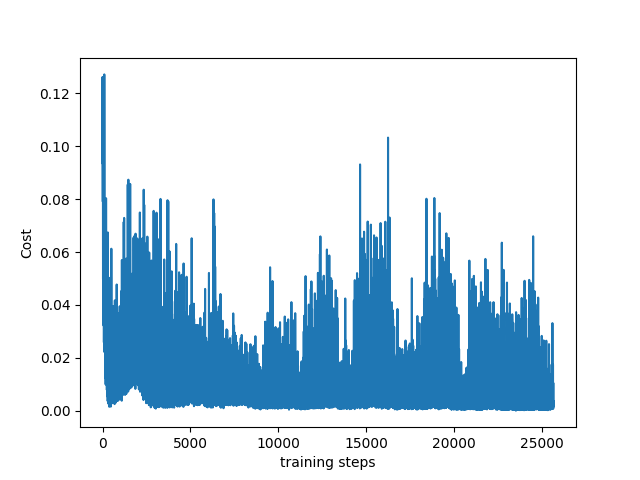
为了将每一步训练的损失值话出来,需要建立一个损失函数:
1 2 3 4 5 6
| def plot_cost(self): import matplotlib.pyplot as plt plt.plot(np.arange(len(self.cost_his)), self.cost_his) plt.ylabel('Cost') plt.xlabel('training steps') plt.show()
|
到这里未知,DQN的模型以及需要的函数就建立完成了。下面进入第二步,导入CartPole-v0的立杆子的环境并对DQN网络模型进行训练。
首先在新建的Python文件中导入gym模块以及建立好的DQN模型,并且导入CartPole-v0:
1 2 3 4 5 6 7 8
| import gym from DQN import DeepQNetwork env = gym.make('CartPole-v0') env = env.unwrapped print(env.action_space) print(env.observation_space)
|
代码中env = env.unwrapped用来解除环境的一些默认限制。打印函数可以看到该环境有两个离散的动作值和四个状态值。
然后实例化建立好的DQN模型:
1 2 3 4 5 6
| RL = DeepQNetwork(n_actions=env.action_space.n, n_features=env.observation_space.shape[0], learning_rate=0.01, e_greedy=0.9, replace_target_iter=100, memory_size=2000, e_greedy_increment=0.001, output_graph=False)
|
最后就是迭代过程:
1 2 3 4 5 6 7 8 9 10 11 12 13 14 15 16 17 18 19 20 21 22 23 24 25 26 27 28 29 30 31 32 33 34 35
| total_steps = 0 for i_episode in range(100): observation = env.reset() while True: env.render() action = RL.choose_action(observation) observation_, reward, done, info = env.step(action) x, x_dot, theta, theta_dot = observation_ r1 = (env.x_threshold - abs(x))/env.x_threshold - 0.8 r2 = (env.theta_threshold_radians - abs(theta))/env.theta_threshold_radians - 0.5 reward = r1 + r2 RL.store_transition(observation, action, reward, observation_) if total_steps > 1000: RL.learn() if done: print('episode: ', i_episode, 'cost: ', round(RL.cost, 4), ' epsilon: ', round(RL.epsilon, 2)) break observation = observation_ total_steps += 1 RL.plot_cost()
|
代码中将状态值作为奖励值,(默认的将离职返回为-1,不适合作为DQN的奖励值。),每一步都要保存状态信息,当总步数大于1000步的时候开始对DQN模型进行训练,前面的步用来收集用于学习的状态信息。
每一次迭代结束之后打印迭代数,损失值,和贪婪值。最后完成100次迭代之后,画出损失值的图。
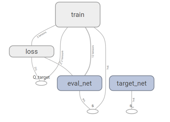
将DeepQNetwork类中的参数output_graph=True,可以在TensorBoard中看到DQN网络的结构图:
参考资料: