本文主要介绍强化学习中Policy Gradients算法的设计与实现过程。
跟上一篇介绍DQN的文章类似,本文也是基于gym环境和TensorFlow来实现来实现Policy Gradients算法,用到的环境也是CartPole-v0的立杆子的环境。具体Policy Gradients的算法过程可以参考之前的文章,今天主要介绍算法的实现过程。
代码同样分为两部分,首先是建立Policy Gradients更新过程,然后建立CartPole-v0环境并对模型进行训练。
涉及的主要模块版本号:
Python:3.5.3
TensorFlow:1.0.1
gym:0.8.1
首先建立Policy Gradients模型。
导入模块和一些初始设置:
1 2 3 4 5 6
| import numpy as np import tensorflow as tf np.random.seed(1) tf.set_random_seed(1)
|
然后定义PolicyGradient类:
1 2 3 4 5 6 7 8 9 10 11 12 13 14 15 16 17 18 19 20 21 22 23 24 25 26 27
| class PolicyGradient: def __init__( self, n_actions, n_features, learning_rate=0.01, reward_decay=0.95, output_graph=False, ): self.n_actions = n_actions self.n_features = n_features self.lr = learning_rate self.gamma = reward_decay self.ep_obs, self.ep_as, self.ep_rs = [], [], [] self._build_net() self.sess = tf.Session() if output_graph: tf.summary.FileWriter("logs/", self.sess.graph) self.sess.run(tf.global_variables_initializer())
|
然后建立网络模型,与DQN的模型类似,在输入和输出之间添加了一个10个隐藏节点的隐藏层。
1 2 3 4 5 6 7 8 9 10 11 12 13 14 15 16 17 18 19 20 21 22 23 24 25 26 27 28 29 30 31 32 33 34 35
| def _build_net(self): with tf.name_scope('inputs'): self.tf_obs = tf.placeholder(tf.float32, [None, self.n_features], name="observations") self.tf_acts = tf.placeholder(tf.int32, [None, ], name="actions_num") self.tf_vt = tf.placeholder(tf.float32, [None, ], name="actions_value") layer = tf.layers.dense( inputs=self.tf_obs, units=10, activation=tf.nn.tanh, kernel_initializer=tf.random_normal_initializer(mean=0, stddev=0.3), bias_initializer=tf.constant_initializer(0.1), name='fc1' ) all_act = tf.layers.dense( inputs=layer, units=self.n_actions, activation=None, kernel_initializer=tf.random_normal_initializer(mean=0, stddev=0.3), bias_initializer=tf.constant_initializer(0.1), name='fc2' ) self.all_act_prob = tf.nn.softmax(all_act, name='act_prob') with tf.name_scope('loss'): neg_log_prob = tf.nn.sparse_softmax_cross_entropy_with_logits(logits=all_act, labels=self.tf_acts) loss = tf.reduce_mean(neg_log_prob * self.tf_vt) with tf.name_scope('train'): self.train_op = tf.train.AdamOptimizer(self.lr).minimize(loss)
|
然后建立动作选择函数:
1 2 3 4
| def choose_action(self, observation): prob_weights = self.sess.run(self.all_act_prob, feed_dict={self.tf_obs: observation[np.newaxis, :]}) action = np.random.choice(range(prob_weights.shape[1]), p=prob_weights.ravel()) return action
|
代码中,在运行网络模型得到动作的权重之前,需要注意一点,就是要将状态值observation添加一个维度再传递给TensorFlow的网络模型中。np.random.choice可以根据p参数给出的概率来选择动作。
然后建立状态存储函数,用来存储状态值,动作值,和奖励值:
1 2 3 4
| def store_transition(self, s, a, r): self.ep_obs.append(s) self.ep_as.append(a) self.ep_rs.append(r)
|
Policy Gradients不需要存储动作的下一个状态值是因为算法在更新的时候直接使用一组完整的状态动作值对,每次学习时前后的状态本身就是有联系的,并不像DQN中采用随机采样的方法来实现。
然后建立学习函数:
1 2 3 4 5 6 7 8 9 10 11 12 13
| def learn(self): discounted_ep_rs_norm = self._discount_and_norm_rewards() self.sess.run(self.train_op, feed_dict={ self.tf_obs: np.vstack(self.ep_obs), self.tf_acts: np.array(self.ep_as), self.tf_vt: discounted_ep_rs_norm, }) self.ep_obs, self.ep_as, self.ep_rs = [], [], [] return discounted_ep_rs_norm
|
每次学习完成之后需要清空存储空间一边下一次训练时从新保存新的状态动作值。
在学习之前需要将奖励值正则化,因此还需要建立奖励值正则化的函数:
1 2 3 4 5 6 7 8 9 10 11 12
| def _discount_and_norm_rewards(self): discounted_ep_rs = np.zeros_like(self.ep_rs) running_add = 0 for t in reversed(range(0, len(self.ep_rs))): running_add = running_add * self.gamma + self.ep_rs[t] discounted_ep_rs[t] = running_add discounted_ep_rs -= np.mean(discounted_ep_rs) discounted_ep_rs /= np.std(discounted_ep_rs) return discounted_ep_rs
|
到此,Policy Gradients的模型已经建立完成。下面就需要导入gym环境对模型进行训练。
同样也需要导入涉及的模块
1 2 3
| import gym from PolicyGradients import PolicyGradient import matplotlib.pyplot as plt
|
然后设置一些基本的参数并导入CartPole-v0环境
1 2 3 4 5 6
| DISPLAY_REWARD_THRESHOLD = 400 RENDER = False env = gym.make('CartPole-v0') env.seed(1) env = env.unwrapped
|
DISPLAY_REWARD_THRESHOLD设置了一个奖励门限,当奖励值大于门限的时候开始显示图形界面,因为奖励值小的时候说明训练效果还不是太好,所以为了节省时间就忽略的界面显示。
然后实例化PolicyGradient:
1 2 3 4 5 6 7
| RL = PolicyGradient( n_actions=env.action_space.n, n_features=env.observation_space.shape[0], learning_rate=0.02, reward_decay=0.99, )
|
最后就是对模型进行训练:
1 2 3 4 5 6 7 8 9 10 11 12 13 14 15 16 17 18 19 20 21 22 23 24 25 26 27 28 29 30 31 32 33
| for i_episode in range(3000): observation = env.reset() while True: if RENDER: env.render() action = RL.choose_action(observation) observation_, reward, done, info = env.step(action) RL.store_transition(observation, action, reward) if done: ep_rs_sum = sum(RL.ep_rs) if 'running_reward' not in globals(): running_reward = ep_rs_sum else: running_reward = running_reward * 0.99 + ep_rs_sum * 0.01 if running_reward > DISPLAY_REWARD_THRESHOLD: RENDER = True print("episode:", i_episode, " reward:", int(running_reward)) vt = RL.learn() if i_episode == 0: plt.plot(vt) plt.xlabel('episode steps') plt.ylabel('normalized state-action value') plt.show() break observation = observation_
|
运行程序可疑看到,当训练迭代到87步左后的时候模型已经达到比较好的效果。
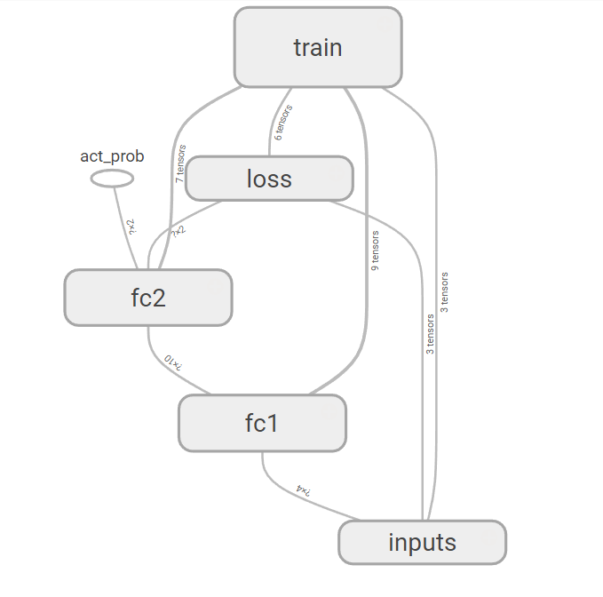
设置PolicyGradient类中的参数output_graph=True,可疑在TensorBoard中看到PolicyGradient网络模型的结构:
参考资料: